Table of Contents
Lecture Notes: FRAP internal course
April 20, 2010 @EMBL
Kota Miura
will also be further added by Sebastian Huet and Christian Tischer
Google Chrome or Firefox (version > 3.6) is recommended for properly viewing math equations.
Introduction
in vivo protein kinetics could be analyzed in two ways: by measuring particular movement or averaged movement. By tracking labeled single protein molecules, we could estimate their diffusion and transport behavior. Such single-molecule studies of membrane proteins, for example, enabled us to analyze how they are organized with their dynamics, such as boundaries for movement constrained by membrane corrals. Motor proteins moving along cytoskeletal tracks were analyzed in detail to know how they convert chemical energy into physical force. This was only possible by probing their singular movement and steps. While single particle tracking requires a high-temporal and spatial resolution setup for analysis, analysis of averaged movement, measured by temporal changes in fluorescence intensity, could be achieved with larger spatial and temporal resolution (typically in micrometer scale).
Here, we focus on one of such averaged movement analysis techniques: Fluorescence Recovery After Photobleaching (FRAP). We first start the explanation with a simpler case of monitoring averaged movement that does not need to bleach.
Fluorescence intensity and Protein Dynamics
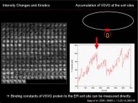
An increase in intensity at the observed area could be measured to know the net increase in the protein at that region. To characterize this dynamics, we can apply traditional biochemical kinetics. Example case: Kinetics of VSVG protein accumulation at the ER exit site.
$${dI(t)\over dt}=k_{on}[VSVG_{free}]- k_{off}[VSVG_{ERES}]$$
Here,
- \(k_{on}\) is the binding rate of VSVG protein to the ER exit site
- \([VSVG_{free}]\) is the concentration of unbound VSVG protein
- \(k_{off}\) is the dissociation rate of VSVG protein from the ER exit site
- \([VSVG_{ERES}]\) is the density of VSVG protein bound to the ER exit site
During the initial phase of binding, when there is almost no VSVG protein bound to the ER exit site, we can approximate that the initial speed of the density increase at the ERES site depends only on the binding reaction: \(k_{off}[VSVG_{ERES}]\simeq0\). \\Then
$$ {dI(t)\over{dt}}=k_{on}[VSVG_{free}] $$
Since there are enough free VSVG, we consider that \([VSVG_{free}]\) is constant; we can simply calculate the slope of the initial increase of intensity, measure the free VSVG intensity, and then calculate \(k_{on}\).
For details, see Runz et al (2006).
FRAP Simple Measures
Unlike the example shown above, protein dynamics are not observable to the eye (through a microscope) in many cases. Even though proteins are exchanging in the system, the flux of protein constituting the system is not evident if the in/out flux of protein is steady and constant (e.g. liver). In such cases, we need to somehow experimentally treat the system. One way is FRAP.
In FRAP, we bleach some population of fluorescence-labeled protein and evaluate the mobility of the protein. Typically, we use confocal microscopy and bleach fluorescence of a small area of the system with a short pulse of a strong laser beam and measure the following changes in the fluorescence intensity at that bleached spot over time. Details on this measurement protocol have been presented in Stefan and Yury's talks (link?). Here, we focus on how to analyze the curve we obtained through such measurements.
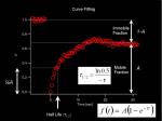
From measured temporal changes in the intensity at the bleached Region of Interest (this curve indeed is the Fluorescence Recovery After Photobleaching, FRAP), we can measure two parameters that represent the speed of recovery and the fraction of molecules moving around in the system.
- Half Max
- Mobile-Immobile fraction
Fitting the curve to an exponential equation allows us to calculate these parameters. Half-Max value (time) is a rather qualitative value, but it is a simple index for comparing different systems.
FRAP Measurements based on Modelling
The FRAP curve reflects the mobility of proteins. In the dilute solution of with a single protein solute, the mobility of the protein could probably be considered as pure diffusion. But in many cases, this does not hold. The mobility is often affected by the system.
- reaction with other proteins
- geometry of the system, which constrains the mobility
- active transport process
By modeling how the mobility is (generate some hypotheses on how the protein mobility is affected in the system), we can set up equation/s to hypothesize what the bases of FRAP curve. To test the hypothesis, we fit the experimental curves with the theoretical curve. By evaluating the goodness of fit, we can discuss which models would be the most likely hypothesis. If the fit is good, then we could know the value of biochemical parameters that govern the recovery curve.
Currently, we have more-or-less standardized protocol to analyze FRAP curves. Starting with a simple model of diffusion, we test the fit of different curves and proceed to more complex models. See the next section for the protocol.
Choosing models based on trial fittings
Maybe Sebastian's flow chart here.
Diffusion Recovery
pure diffusion
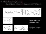
The theoretical curve of the diffusion-mediated fluorescence recovery was proposed by Soumpasis (1984) and has been widely used.
$$
f(t)=e^{- \frac{\tau_D}{2t}}\left(I_{0}(\frac{\tau_D}{2t})+I_{1}(\frac{\tau_D}{2t})\right)
$$
This theoretical equation assumes:
- 2D
- circular (cylindrical) bleaching
When the above equation could be fitted nicely (evaluated by goodness of fit, such as Pearson's coefficient r or gamma-Q value), one could calculate the diffusion coefficient by using the obtained $\tau_D$ and radius of the circular ROI \(w\).
$$
D=\frac{w^{2}}{\tau_D}
$$
For strip-ROI bleaching, the empirical formula used by Ellenberg et al. (1997) could be used, and it is also possible to use Gaussian curve fitting that Christian Tischer developed. For Christian's method, 100426FRAPgaussfit.
effective diffusion
(almost diffusion)
anomalous diffusion
Reaction Dominant Recovery
If the molecule under study is binding/unbinding with other molecular species, the FRAP curve is affected by these interactions. There are two cases on how these two events, diffusion and reaction, are combined in the curve. We could think of two cases.
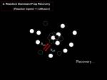
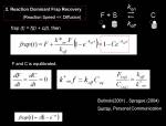
- Reaction-dominant recovery Cases when reaction binding rate (meaning “number of molecules that bind to the binding partner per second”) is much lower than the diffusion rate. In such cases, the FRAP-bleached field will first become brighter due to diffusion, and then there will be a slower recovery of intensity due to non-bleached fluorescence exchange with the bleached fluorescence. In such cases, we could consider that the recovery curve is dominated by reaction since the duration of the diffusion-recovery phase is much shorter compared to the reaction-recovery phase. In such a case, these two phases are considered to be separable (call this reaction-dominant or diffusion uncoupled; this section). We might not even “see” the diffusion recovery phase, which requires high temporal resolution capturing.
- Reaction-Diffusion Recovery Other cases would be when durations of diffusion-recovery phase and reaction-recovery phase are with comparable duration. Then recovery curve consists of a combination of fluorescence that came in with diffusion, and also by the binding of fluorescence molecule at the FRAP bleached field (“reaction-diffusion” or “diffusion-coupled” see the section below).
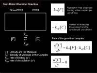
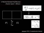
For a simple chemical reaction with a singular type of interaction, we could again think of the reaction model that was already explained above, the first-order chemical reaction modeled as a compartment system (see figure right)
$$
\frac {df(t)} {dt} = k_{on}[free] - k_{off}[bound]
$$
where
- \(k_{on}\) Binding constant
- \(k_{off}\) Dissociation constant
- \([free]\) Density of free molecules
- \([bound]\) Density of bound-molecules
We solve the differential equation $$ f(t)=A(1-e^{- \tau t}) $$ where
- \(\tau = k_{on} + k_{off}\)
- \(A = \frac {k_{on}}{k_{on} + k_{off}}\)
Reaction Dominant Recovery with Immobile Binding Partner
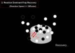
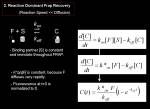
Next we modify above model to consider a situation a bit more frequently we see in cell biology. The protein we are analyzing is either freely diffusing in cytoplasm or bound to an immobile structure inside cell. We FRAP this structure, to know the kinetic constants of the protein interaction with the structure (e.g. microtubule binding protein, structure = microtubule) $$ \frac {df(t)} {dt} = k_{on}[free][s] - k_{off}[bound] $$ where
- \(k_{on}\) Binding constant
- \(k_{off}\) Dissociation constant
- \([free]\) Density of free molecules
- \([s]\) Density of immobile binding partner
- \([bound]\) Density of bound-molecules
Since [s] is immobile and constant during the experiment, we define \(k*_{on}\) as $$ k*_{on}=k_{on}[s] $$ In addition, the density of free molecules in cytoplasm is almost constant, so we assume \([free] = F\) and does not change. We then solve $$ \frac {df(t)} {dt} = k*_{on}F - k_{off}[bound] $$ We get $$ f(t)=1-Ce^{- \tau t} $$ where
- \(\tau = k_{off}\)
… note that the shape of the recovery curve now only depends on \(k_{off}\)
Diffusion and Reaction combined Recovery
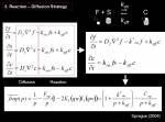
$$ \frac{\partial [free]}{\partial t} = D_{free} \nabla ^2[free]-k_{on}[free][s]+k_{off}[bound] $$ $$ \frac{\partial [s]}{\partial t} = D_s \nabla ^2[s]-k_{on}[free][s]+k_{off}[bound] $$ $$ \frac{\partial [bound]}{\partial t} = D_{bound} \nabla ^2[bound]+k_{on}[free][s]-k_{off}[bound] $$
Since
- [s] is constant and immobile
- \(k*_{on} = k_{on}[s]\)
- \(\frac{\partial [s]}{\partial t}=0 \)
- bound molecules do not diffuse so \(D_{bound}=0\)
Then we solve only $$ \frac{\partial [free]}{\partial t} = D_{free} \nabla ^2[free]-k*_{on}[free]+k_{off}[bound] $$ $$ \frac{\partial [bound]}{\partial t} = k_{on}[free][s]-k_{off}[bound] $$
We could solve this either analytically (Sprague et al, 2004) or numerically (Beaudouin et al, 2006). In the latter paper, the calculation involves spatial context (on-rate was spatially varied; see also the “geometry” section below).
Sprague Method
An analytical solution was made in the Laplace transform equation. $$ \overline{frap(p)} = \frac 1 p - \frac{F_{eq}}{p}\left(1-2K_1(qw)I_1(qw)\right)\times\left(1+\frac{k*_{on}}{p+k_{off}}\right)-\frac C {p+k_{off}} $$
Beaudouin Method
Diffusion and Transport combined Recovery
We did not talk about this issue in the course, but there is another factor that could interfere with the recovery curve in vivo: active transport. There is a trial on including this factor by Hallen and Endow (2009).
Diffusion and Reaction, along with Spatial Context, Geometry
Since molecular behavior inside the cell is constrained largely by the structure and geometry of intracellular architecture, FRAP measured at a single point within a cell does not always represent the biochemical characteristic of that molecule. The functionality of a protein molecule is determined not only by switching on/off, but is also regulated by the position of that molecule within the cell. This means that spatial context should be included when interpreting the FRAP measurement.
Physical parameters such as the Diffusion coefficient measured by FRAP are affected largely by geometrical constraints. Even if the geometry is rather simple, there are many obstacles in the intracellular space that will cause a longer time for molecules to reach from one point to the other. In such cases (which is probably frequently the case), the estimated diffusion coefficient would be calculated to be smaller than that of the “true diffusion coefficient”. The presence of such obstacles should be taken into account. For this reason, estimation of the Diffusion coefficient could be more precise if one analyzes the structural geometry of where the molecule is constrained. Such a protocol would be especially important if the Diffusion and reaction-coupled recovery curve, since wrong estimates of the Diffusion coefficient would end up in wrong reaction parameters as well.
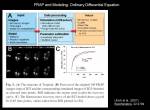
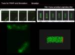
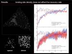
Joel Beaudouin, who did his PhD study in the Ellenberg lab in the EMBL, encountered such a question in his project on nuclear protein study and solved the problem by using initial image frames of the FRAP experiment and let the molecule to diffuse by simulation, then fit the simulation with the experimental FRAP image sequence. Diffusion-reaction model was used, and a simulation was done (see above) using an ODE solver to scan through the parameter space. Excellent idea. For more details, see Beaudouin et al. (2006). We will later add some protocol to these lecture notes on how to fit FRAP image sequence data using an ODE solver (with the help of Sebastian Huet). Joel's method was made into an application called “Tropical” by a team at the University of Heidelberg, but it seems that there is no direct link for downloading.
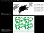
Other papers we could refer to are Sbalzarini et. al. (2005, 2006). In these papers, authors did two things in parallel: 3D reconstruction of ER membrane structure and FRAP of a certain molecule moving around along ER membrane. Using the 3D structure they reconstructed, geometrical constraints on protein diffusion could be determined and included this constraint on the estimation of the Diffusion coefficient.
Pitfalls in FRAP Analysis
Refer to Mueller et. al.(2008). In their paper, they pointed out
- Shape of the FRAP ROI largely affect estimated value of biochemical rate constants(diffusion is important)
- Problems of fitting double exponential curve
- Initial condition (laser intensity profile) is important
- “blinding” of photomultiplier after the FRAP bleaching
List of Tools for FRAP Analysis
Basic
- ImageJ Plugins: Two available ImageJ plugins for FRAP does intensity measurement and normalization. Fitting module is not implemented.
- There is a good step-by-step protocol for measurements and analysis using MBF ImageJ bundle. You need to download the bundle from the linked site, and also ask for some plugins directly by email.
- FRAP analysis (EMBL)
- Import data output from Zeiss, Leica, Olympus measurements and do FRAP fitting.
- FRAP analyzer (University of Luxemburg)
- Similar to above, but stand alone and also incorporated diffusion-reaction model.
-
- Does measurement and fitting. Sprague et al. (2004) Reaction-Diffusion Full model is implemented.
Two Advanced strategies: Analytical and Numerical Approaches
Requires your own coding, customization
Analytical Approach
Sprague et. al. (explained above) is an example case of analytically solving the model for the fitting.
ODE Simulation
Tropical
- Numerical analysis based on ODE. Spatial context.
General Solvers
-
- Joel and Sebastian uses this software for fitting ODE.
Particle Simulation
Particle Simulation Packages
- Smoldyn
- GridCell
- MCell
References recommended
Reviews, Protocols and textbooks
- McNally, J.G. (2008) Quantitative FRAP in analysis of molecular binding dynamics in vivo. Methods in Cell Biology 2008;85:329-51
- step-by-step protocol for analyzing FRAP. Flow chart for determining recovery model is useful.
- Sprague, B. L. and McNally, J. G.(2005). FRAP analysis of binding: proper and fitting. Trends Cell Biol 15, 84-91.
- Phair, R. D., Gorski, S. A. and Misteli, T. (2004). Measurement of dynamic protein binding to chromatin in vivo, using photobleaching microscopy. Methods Enzymol 375, 393-414.
- Already a bit of out-dated but “Double normalization” introduced in this protocol is widely used.
- Jacquez, J. A. (1972). Compartmental analysis in biology and medicine: Elsevier
- If you want to study basics about calculation of kinetics.
Research Papers
- Soumpasis, D. M. (1983). Theoretical analysis of fluorescence photobleaching recovery experiments. Biophys J 41, 95-7.
- Fitting 2D diffusion, circular ROI bleaching.
- Sprague, B. L., Pego, R. L., Stavreva, D. A. and McNally, J. G. (2004). Analysis of binding reactions by fluorescence recovery after photobleaching. Biophys J 86, 3473-95.
- details on analytical approach for full diffusion-reaction model.
- Sbalzarini, I.F., A. Hayer, A. Helenius, and P. Koumoutsakos. (2006) Simulations of (an)isotropic diffusion on curved biological surfaces. Biophys J. 90:878-85.
- Sbalzarini, I.F., A. Mezzacasa, A. Helenius, and P. Koumoutsakos. (2005) Effects of organelle shape on fluorescence recovery after photobleaching. Biophys J. 89:1482-92.
- papers which revealed that spatial and geometrical factors are very important for the interpretation and analysis of FRAP curves.
- Beaudouin, J., Mora-Bermudez, F., Klee, T., Daigle, N. & Ellenberg, J.(2006) Dissecting the contribution of diffusion and interactions to the mobility of nuclear proteins. Biophys J. 2006 Mar 15;90(6):1878-94.
- full reaction-diffusion fitting by numerical approach, with spatial context
- Ulrich M, Kappel C, Beaudouin J, Hezel S, Ulrich J, Eils R.(2006)Tropical–parameter estimation and simulation of reaction-diffusion models based on spatio-temporal microscopy images. Bioinformatics. 22(21):2709-10
- Mueller F, Wach P, McNally JG.(2008) Evidence for a common mode of transcription factor interaction with chromatin as revealed by improved quantitative fluorescence recovery after photobleaching. Biophys J. 2008 Apr 15;94(8):3323-39
- Pitfalls on FRAP analysis. You will be shocked by how problematic it could be…
