Python Image Processing Cookbook

matplotlib has matplotlib.image.imread, and PIL also has similar file input methods. The former is limited to png files and the latter is limited to 8-bit images. For this reason, we focus on openCV and TiffFile modules.

>>> import cv
>>> img = cv.imread('/Users/miura/img/blobs.tif')
>>> type(img)
>>> <type 'numpy.ndarray'>

• cv.imread reads only the first frame in tiff stack.
• 8bit image becomes RGB-like format, triplet of 8 bits per pixel.

In [40]: img = cv.LoadImage('/Users/miura/img/blobs.tif')
In [41]: img
Out[41]: <iplimage(nChannels=3 width=256 height=254 widthStep=768 )>

In [44]: import tifffile as tff
In [50]: tiffimg = tff.TIFFfile('/Users/miura/img/blobs.tif')
In [51]: type(tiffimg)
Out[51]: <class 'tifffile.TIFFfile'>
In [52]: img = tiffimg.asarray()
In [53]: type(img)
Out[53]: <type 'numpy.ndarray'>

In [54]: tiffimg = tff.TIFFfile('/Users/miura/img/flybrainG.tif')
In [55]: img = tiffimg.asarray()
In [57]: tiffimg
Out[57]: <tifffile.TIFFfile object at 0x1299ac910>
In [65]: type(img)
Out[65]: <type 'numpy.ndarray'>
In [61]: img10 = tiffimg[10].asarray()
In [62]: type(img10)
Out[62]: <type 'numpy.ndarray'>

• if the image file is a single frame image, not so different from the others
• Stack tiff file is loaded peroperly. Single frame is extractable by indexing. In above case, 11th frame is extracted.

• tested with python2.6, openCV 2.2, numpy 1.6.1, OSX10.6.8

>>> import cv
>>> import numpy as np
>>> mat = cv.CreateMat( 3 , 5 , cv.CV_32FC1 )
>>> cv.Set( mat , 7 )
>>> a = np.asarray( mat[:,:] )
>>> a
array([[ 7.,  7.,  7.,  7.,  7.],
       [ 7.,  7.,  7.,  7.,  7.],
       [ 7.,  7.,  7.,  7.,  7.]], dtype=float32)

<link>

• tested with python2.6, openCV 2.2, numpy 1.6.1, OSX10.6.8

>>> im = cv.CreateImage( ( 5 , 5 ) , 8 , 1 )
>>> cv.Set( im , 100 )
>>> im_array = np.asarray( im )
>>> im_array
array(<iplimage(nChannels=1 width=5 height=5 widthStep=8 )>, dtype=object)
>>> im_array = np.asarray( im[:,:] )
>>> im_array
array([[100, 100, 100, 100, 100],
       [100, 100, 100, 100, 100],
       [100, 100, 100, 100, 100],
       [100, 100, 100, 100, 100],
       [100, 100, 100, 100, 100]], dtype=uint8)

<link>

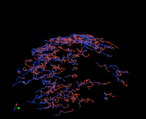
An example script for loading (x, y, y) coordinates data from tab-delimited text file and plot them in 3D using mayavi2.

from matplotlib import mlab as matp
filename = '/Users/miura/data.txt'
x1, y1, z1, x2, y2, z2 = matp.load(filename, usecols=[0, 1, 2, 3, 4, 5], unpack=True)

from mayavi.mlab import points3d
from mayavi.mlab import plot3d
from mayavi import mlab as maya

p1s = points3d(x1, y1, z1, scale_factor=.25, color=(0, 1, 1))
p2s = points3d(x2, y2, z2, scale_factor=.25, color=(1, 0, 0))

for idx, xval in enumerate(x1):
    plin1 = plot3d([x1[idx], x2[idx]], [y1[idx], y2[idx]], [z1[idx], z2[idx]], tube_radius=0.1, colormap='Spectral', color=(0, 0, 1))
maya.show()

plotting data with mayavi

In this example, we assume the follwoing data structure in the file: a pair of coordinates per line, so 6 numbers are in one line separated by tab. It should look like

1.0 3.6 4.8 5.1 6.12 7.14
...  

To run this script, the best is to run it from ipython with thread so first you start ipython by

ipython -wthread

or incase of newer ipython (version >= 1.1)

ipython --i

then in the ipython interface,

run exampleMayavi.py

A new window pops up, and after drawing of the scene is finished, you could control the scene by such as

maya.view(100, 40)

or to animate the scene

for i in range (1, 360, 3): maya.view(i, i)

to close the scene,

maya.close()

Note that in this example,

from mayavi import mlab as maya

since the namespace “mlab” overlaps with matplotlib.mlab.

To evaluate 3D particle tracking results, trajectories could be plotted by color coding the time.

Plotting 3D trajectory. Trajectories are colored so that the beginning of frame is blue and gradually become red towards the end of the sequence