A

For a simple comparison of several different experiment results, interpretation of FRAP (Fluorescence Recovery After Photobleaching) curves can be qualitative. Just by looking at the graph the speed of recovery to the plateau intensity can be examined. For example, Figure 1-1 shows several FRAP curves derived from cells under different treatments.

$Text Box: Figure 1-2 Frap Curve and its parameters: Mobile fraction (a), immobile fraction (b) and half maximum tau (d)$ Text Box:

Figure 1-1
Example FRAP curves (courtesy of Heiko Runz). The recovery of blue curves is faster than the red curve. We can then say that the mobility of the observed molecule is faster in the blue curve condition than the red curve condition. The plateau level seems to be also different in two conditions. Blue curve plateau is higher than that of the red curve. We then know that the mobile fraction (see below) of the molecule is larger in the blue conditions than in the red condition.

To add a bit more quantitative taste, we can measure these two features (recovery speed and recovery fraction) numerically from the FRAP curves. An example of actual FRAP curve after normalization is shown in Figure 1-2.

In many cases FRAP recovery curves do not always reach the level of original fluorescence intensity. In Fig. 1-2 a, the plateau level is lower than the pre-bleach fluorescence intensity because some of the FRAP-bleached molecule are immobile within the FRAP ROI that they do not contribute to the recovery and at the same time do not give away free binding sites for incoming un-bleached proteins. For these reasons, fraction of proteins that contribute to the recovery are called ‘mobile fraction’ and those do not are called ‘immobile fraction’. Each corresponds to a and b (=1-a) in figure 1-2, respectively. Conventionally used index for the speed of recovery is the time it takes for the curve to reach 50% of the plateau fluorescence intensity level (c) and is called ‘half maximum’ or ‘half life’ and often abbreviated as ‘τ_1/2’(d, tau half). Shorter half max tells us that the recovery is faster.

A more objective way to extract half max and mobile / immobile fraction is to fit the normalized FRAP curve I(t) by an exponential equation

(1-1)

The fitted coefficients can be used for calculating following parameters of the FRAP curve:

Mobile fraction = A (1-2)

Immobile fraction = 1-A (1-3)

Half Max: (1-4)

1.2. Quantitative Interpretations (Not Finished!)

For any kind of molecules within biological system, two major factors affect their mobility. First is diffusion. Diffusion of the molecule drives the change in the position of the molecule from time to time. Rate of diffusion is determined by the diffusion constant of the molecule, which is affected by the size of the molecule, viscosity and temperature of the surrounding medium. Physical structures that hinder their pure diffusion can also be considered as another factor and can be considered as a parameter for the apparent viscosity of the medium (cf. Luby-Phelps). Second is the chemical interaction. The environment of molecule is rarely a pure solvent in biological system. These surrounding molecular species interact with the observed molecule. Binding and dissociation, namely the binding constants of the molecule with others, affects the mobility of the molecule. Therefore FRAP recovery curve is determined by two major factors.

If the diffusion of the molecule is fast and the interaction of molecule is slow, then the rate limiting factor for the mobility is the interaction. In this case, we assume that the FRAP recovery curve is dominated by the chemical interaction. If the interaction of the molecule is faster than the diffusion, then the mobility of the molecule is dominated by the diffusion.

Choice of equation for fitting the recovery curve of FRAP experiments depends on what you assume for the mobility of the protein that you are studying. There are three different models. (1) Chemical Interaction Model (2) Diffusion Model (3) Reaction-Diffusion model.

1.2.1 Chemical Interaction Models

FRAP curves are fitted with exponential equation in chemical interaction models,. In the simplest case, the equation is with a single exponential term and called “single exponential equation” and was already introduced above as the equation (1-1).

The exponential equation is an analytical solution of a two-compartment model (Jacquez, 1972). We consider molecule in one chamber A. The concentration of the molecule is [A] and the molecule is moving to the neighboring chamber B though a narrow channel that connects two chambers as shown in the illustration below (Figure 3.).

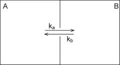
Figure 3. Compartmental Model of a Simple Chemical Interaction

If the rate constant of transition from A to B is ka and from B to A is kb, then the rate of the change of the molecule concentration in the chamber B is

(1-5)

Solving this equation using parameter variations and assuming that [B]=0 when t=0, yields exponential equation (1-1) with

(1-6)

(1-7)

The interaction of observed molecule is not necessarily limited to a single interaction. If the molecule we are observing possesses two independent binding sites, then there are two interactions.

Although the interactions are independent, we observe fluorescence recovery that is sum of these two interactions and the analytical solution would be a double exponential equation (see below).

Double exponential equation arises also in other cases. For example, the interaction could be in two steps such that the molecule interacts first weakly, and then upon this weak interaction will there be a strong interaction.

K_a, K_b, K_c and K_d are rate constants. Although the state of interaction is different, binding in weak and strong forms both contribute to the recovery of the fluorescence. Thus the recovery curve is

(1-8)

Since source of fluorescence outside the FRAP ROI is enormous, we assume that [A] is always constant.

(1-9)

[B_w] and [B_s] increases with time. The rates of increase of the molecule with each binding state are

(1-10)

(1-11)

Solving these coupled differential equations, we obtain a double exponential equation

(1-12)

y₀=A₁+A₂(1-13)

1.2.1.2 Chemical Interactions with immobile entity.

(Recovery depends only on Koff. Refere to Sprague et al. 2004)

1.2.2. Diffusion models

There are two formulas proposed for fitting the diffusion-limited FRAP recovery curves. Soumpasis modified the initial formula proposed by Axelrod et al. (1974) as follows:

(Soumpasis, 1983)

This formula is purely theoretical.

Ellenberg et al. proposed an empirical formula as below.

(Ellenberg et al., 1997)

Details of the parameters used in these equations will be discussed later. Note that the shape of the FRAP-ROI affects the recover kinetics largely. Each fitting equation assumes certain shapes for the FRAP-ROI. The area of the FRAP-ROI also matters so you must do the experiment with a constant FRAP-ROI area.

1.2.3 Reaction-Diffusion Models.

Any molecular mobility has both Reaction and diffusion components. Above two models are simplifies this reality by assuming that one of these two components is negligible. Logically including both components would be the ultimate direction of the modeling-based fitting (Sprague and McNally, 2005; Sprague et al., 2004). This model is not implemented yet in the program.

2. Analysis of FRAP curves in Practice

2.1 Data Requirements for Precise Measurements of Molecular Dynamics by FRAP

Following four different regions are recommended to be measured for each experiment (see Figure 4).

(1) FRAP ROI (ROI=Region Of Interest). Region where you actually bleached the fluorophore by strong laser irradiation. Shape and size of the bleaching must be controlled. Shape of the FRAP ROI, circular, rectangular, affects the model equation to be fitted with. Size of the ROI matters with the diffusion-limited type of FRAP recovery (see below).

(2) Reference ROI Also called ‘Cell Part’. ROI within the same cell (or it could be other cell) to measure a decay in fluorescence due to the acquisition bleaching. The result could be erroneous (see xx for more explanation).

(3) Base ROI Also called ‘background’. Set ROI outside the cell, where there should be no fluorescence, to know the offset intensity.

(4) Whole Cell ROI or ‘All cell’. The average fluorescence intensity of the whole cell you are observing.

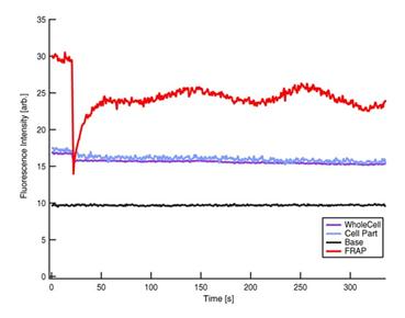
Figure 4 Fluorescence intensity kinetics at four different positions (courtesy of Mei Rosa Ng).

Red: FRAP, Blue: Part of cell, Purple: Whole Cell and Black: Base line

The minimal data set for measuring the proper kinetics is FRAP ROI (1) and BASE ROI(4). It is possible to estimate the recovery kinetics without (4), but if the baseline is high relative to the signal and different from one another experiments, the interpretation of data deviates largely from the reality. Complete set of data is all four different ROI.

During experiment, we recommend to take more than 20 frames before FRAP bleaching. This is because during the initial acquisition phase fluorescence intensity bleaches largely and FRAP bleaching is better be not overlaid to this systematic bleaching. In addition, for the purpose of estimating “Gap Ratio” which indicates how much o total fluorescence in the system you are observing is lost by FRAP bleaching, pre-bleaching acquisition is better be longer. If you see flat fluorescence intensity curve during pre-bleach, it should be fine. Furthermore, when the program evaluates the goodness-of-fit, since standard deviation error of each time point is in general cases not possible to estimate, the program uses fluctuation of measured intensity during pre-bleach period to estimate “measurement error” and is used for the calculation of gammaQ value. For all these reasons, longer prebleach acquisition is strongly recommended.

2.2 Terms

For numerical treatments of FRAP recovery curves, several technical terms are used. See also Figure 5 and 6.

1. Intensity measurements from different ROIs

FRAP ROI: I_frap(t)

Reference ROI: I_ref(t)

Base ROI: I_base(t)

Whole Cell ROI: I_whole(t)

2. Intensity of FRAP ROI at bleaching time point t_bleach is termed ’frap-bleach intensity’ or I_frap-bleach.

I_frap-bleach= I_frap(t_bleach)

3. Pre-bleach Intensities

Average fluorescence intensity before FRAP bleaching is obtained by first subtracting the off-set fluorescence intensity (base ROI intenisty) from other curves[1] and averaging the value for pre-bleach period:

- FRAP pre-bleach intensity: I_frap-pre

- Reference pre-bleach intensity: I_ref-pre

- Whole Cell pre-bleach intensity: I_whole-pre

- Whole Cell post-bleach intensity: I_whole-post

Average intensity of the Whole cell ROI after the bleaching. Use 10 time points after the bleaching.

f_prebleach is the frame (sampling) number during pre-bleach period.

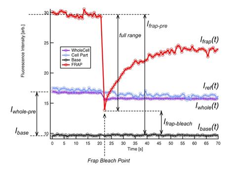
4. ‘Full Range’ is the difference between I_frap-pre and I_frap-bleach.

Figure 5 Terms used in FRAP recovery curve analysis

5. The ratio I_whole-post / I_whole-pre is called ‘gap ratio’ (see Figure 6). This ratio is an indicator of the amount of fluorescence that is lost form the cell by FRAP-bleaching. See section 2.6 ‘Gap Ratio: Effects of FRAP bleaching on un-FRAPped region’ for details.

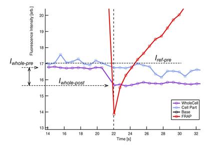
Figure 6 Terms used in FRAP recovery curve analysis

2.3 Normalization of the Frap Curve

Any FRAP curve contains two components of fluorescence intensity changes. The major component is the recovery of fluorescence due to the flux of labeled proteins into the FRAP ROI. The second component is the bleaching of fluorescence everywhere within the microscope field where illumination light is irradiated to excite the fluorophore for measuring their intensity –although very slow, acquisition bleaching causes less and less molecules with fluorescence with time. This acquisition bleaching attenuates the fluorescence recovery, because bleached molecules by this reason also move into the FRAP ROI and attenuate the recovery of fluorescence. Thus, how to correct for acquisition bleaching is one of the key point for the analysis of FRAP curve. In some cases, this correction is included in the normalization procedure but in other cases correction is independent from the normalization procedure. In this latter case, correction will be done by including acquisition bleaching parameters to the FRAP equation for fitting to the measured recovery curve. In the following, I will describe different methods for doing normalizations.

2.3.1. Normalization that involves acquisition bleaching correction This method is known as ‘the double normalization’ (Phair et al., 2004). In double normalization, we take the measurement from whole cell ROI for correcting the acquisition bleaching effects. Average pre-bleach whole cell intensity divided by the whole cell intensity at each time points in the post-bleach period will be multiplied to the FRAP curve at that time point. Before this operation, both Whole Cell ROI and FRAP ROI data are subtracted by Base ROI intensity.

(2-1)

In the ‘single normalization’ method proposed by Phair et al., FRAP curve is simply subtracted by the offset intensity outside of the cell (Base ROI), and then the base intensity is taken as 0 and pre-bleach intensity I_frap-preof the FRAP curve is taken as 1. If whole cell ROI or reference ROI data is not available, then the single normalization method is employed but one should be aware that this does not correct for the acquisition bleaching.

(2-2)

In these methods, FRAP curves are normalized to I_frap-pre that I_frap-bleach >0. For fitting equations that assumes I_frap-bleach=I_frap(t_bleach)=0, such as for diffusion-dominant models ‘Ellenberg’ and ‘Soumpasis’, (2-2) will be further normalized to the full scale.

(2-3)

2.3.2. Normalization that does NOT involve acquisition bleaching correction The FRAP curve is simply normalized by taking pre-bleach fluorescence intensity as 1 and bleach intensity 0.

(2-4)

In this method, Base ROI measurement is not required. Acquisition bleaching will be corrected directly when the curve is fitted, by using parameters for the acquisition bleaching independently acquired through fitting the background decay curve. For more detail, see ‘2.4 Determination of acquisition bleaching parameters’. Following two methods uses this normalization method.

Rainer’s Method

Back Multiply Method

In ‘Rainer’s method’, the background decay curve (either Whole Cell ROI or Reference ROI) will be normalized in the same way as the FRAP ROI.

(2-5)

This calculation may result negative values for the normalized background decay curve but this does not affect the decay parameter. In case of ‘Back Multiply’ method, normalization procedure takes two steps. First, normalize the background curve by

(2-6)

then normalize to the full range by

(2-7)

2.4 Determination of acquisition bleaching parameters

For obtaining parameters of acquisition bleaching, we assume that the decay of fluorescence intensity follows standard exponential decay.

(2-8)

thus

(2-9)

We fit the measured fluorescence decay to the equation (2-9). As the t approaches infinity, fluorescence level approaches to the base line level y_0-decay since all fluorescence will be bleached by time. In case when Whole Cell ROI data is available, then I_whole(t) will be fitted. If not, then Reference ROI data I_ref(t) will be used.

Figure 7 Different Patterns of exponential curves

One practical problem that you may encounter is fitting failure, which will be reflected in the resulted parameters. There could be four combinations for A_decay and τ_decay. See Figure 7 for the shape of each curve.

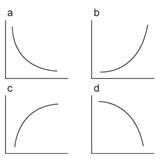
	*A_decay*	*τ_decay*
(a)	+	+
(b)	+	-
(c)	-	+
(d)	-	-

Among these combinations, the fitting is successful only when both parameters are positive (a). (b) and (c) parameter combinations results if the decay curve is an increase in the fluorescence intensity by time, indicating that the quality of the measurement is bad. Double negative parameters (d) results only when the curve has downward curvature, which does not happen for the fluorescence decay by acquisition bleaching. For these reasons, when the parameter combination is not double positive (a), the program automatically sets the background flat and will be indicated in the ‘History’ window. One cause for such problems in the fitted curve could come from the data close to the FRAP bleaching time point since they tend to be unstable. You could avoid fitting those time points. Such an option is implemented in the program (adjust “Back Start”).

2.5. Gap Ratio: Loss of fluorescence due to the FRAP bleaching [2]

When relatively large part of the sample is irradiated for FRAP bleaching, total fluorescence level within the cell will decrease significantly (see Figure 6) by FRAP bleaching. If you are also monitoring other part of the cell by Reference ROI, although the decrease is more gradual, you may detect it as well, because FRAP-bleached molecules moved to the Reference ROI and lowered its fluorescence level (figure 6). The acquisition bleaching which you are observing then contains two components. (a) Bleaching due to illumination light and (b) FRAP bleached molecules moving into the ROI. Effect (b) is a complicated issue. The distance between FRAP ROI and Reference ROI matters with kinetics e.g. closer the distance between two regions, faster that you will detect the decrease. Percentage of the fluorescence that you bleached for FRAP also matters. If the FRAP-bleaching affects the decay of the reference ROI within the cell too much[3], you need to obtain the acquisition bleaching kinetics from the whole cell. If the effect of FRAP-bleaching on the reference point intensity dynamics is minimal e.g. FRAP-bleached fluorescence is negligible against the total fluorescence of the cell, then you can use the reference ROI for acquisition bleaching correction.

We estimate the amount of fluorescence loss due to the FRAP bleaching by obtaining the ‘Gap Ratio’. This value enables us to calculate more precise mobile / immobile fraction of the molecule.

(1) When you have ‘Whole Cell ROI’ data[4]

If you have average fluorescence intensity changes of the whole cell ROI, then the decrease fluorescence by FRAP bleaching will be calculated by taking the ratio of I_whole-pre and I_whole-post.

(2-10)

(2) When ‘AllCell’ data is NOT available[5]

First, we estimate the decay kinetics by fitting the equation (2-9) to post- FRAP bleaching period of I_ref(t). Then we estimate the average fluorescence level before the FRAP bleaching by extrapolating the fitted decay curve[6]. This is an estimation from the intensity changes after the loss of fluorescence by FRAP bleaching, so we call this fluorescence level I_ref-pre-est. From the experiment, we know the measured fluorescence level before the FRAP bleaching. We average these values and we call it I_{ref-pre-measured}. I_back-pre-est is smaller than I_{back-pre-measured} because there is a loss in fluorescence due to the FRAP bleaching. Taking the ratio between these two values, we obtain the Gap Ratio.

(2-11)

We use this Gap Ratio for calculating mobile and immobile fraction. The FRAP curve reaches plateau and we detect this plateau level to know the mobile fraction. However, the plateau level never becomes 1 because we bleached certain fraction of molecules by FRAP bleaching, the fraction which is equal to the Gap Ratio. Hence, we calculate the actual mobile fraction by

MobileFraction_est= MobileFraction_measured / Gap Ratio (2-12)

2.6. Fitting Procedure

2.6.1 Single Exponential – Phair’s double normalization

After normalizing and correcting for the acquisition bleaching, FRAP curve is fitted with standard exponential equation as explained in the “chemical interaction dominant” model.

(2-13)

At bleaching time point, I(t_bleach) = y₀+A and the plateau of the curve is y₀. Mobile fraction will be calculated by

(2-14)

and Half-Max calculation is same as the equation (1-4).

2.6.2 Single Exponential - Rainer’s Method

The rate of fluorescence recovery is proportional to the available binding sites within the bleached region. Simultaneously the recovery rate is attenuated by fluorescence decay due to acquisition bleaching. This attenuation is proportional to the fluorescence level at each time point. Taken together, the rate of fluorescence recovery is

(2-15)

I_max is a fluorescence intensity corresponding to the maximum available binding site. I_max = I_frap-pre if all molecules are mobile. is a time constant characteristic to fluorescence recovery, and is a time constant that characterizes acquisition photobleaching. Solving the differential equation (2-15) and taking that I_frap(t_bleach) = 0,

(2-16)

where,

(2-17)

We obtain before these fittings by fitting post-bleach period of Whole Cell ROI or Reference ROI data as explained in details already (see 2.3) and use it as a constant value during fitting. The estimation curve corrected for the acquisition bleaching will then be

(2-18)

For knowing the mobile – immobile fraction, we consider the Gap Ratio as it was already explained (see 2.5 for more detail).

(2-19)

Half-Max calculation is the same as the equation (1-4) using.

2.6.3 Single Exponential - Back Multiplication Method

The principle of correction for acquisition bleaching is the same as Phair’s method, but instead of scaling each time point of I_frap(t) by corresponding time point I_whole(t) or I_ref(t), we use three parameters of decay curve for directly fitting the un-corrected FRAP curve. The advantage of this method over Phair’s method is that the amplification of error due to multiplication of two data from each time point does not occur. Amplified error will cause lowering of the Gamma-Q value for the evaluation of the fitting (see 2.7). We fit the normalized, uncorrected FRAP curve by following equation.

(2-20)

, y₀, B are obtained by fitting the decay curve, either Whole cell ROI or Reference ROI, that is normalized by the procedure explained already (see 2.3). These three values are taken as constant values during fitting. The estimation curve corrected for the acquisition bleaching will then be

(2-21)

Since decay curve parameters used in (2-20) is the ones from already normalized decay curve, we do not need to consider the Gap Ratio for knowing the mobile fraction.

Mobile = A (2-22)

Half-Max calculation is the same as the equation (1-4) using.

2.6.4. Phair’s Double Exponential Fitting

Similar to the single exponential fitting, we fit the FRAP curve by

(2-23)

At bleaching time point, I(t_bleach) = y₀+A₁+A₂ and the plateau of the curve is y₀. Mobile fraction will be calculated by

(2-24)

2.6.5. Soumpasis Diffusion Fitting

We fit double-normalized FRAP curve as explained already (see 2.3) to the theoretical formula for diffusion FRAP curve

(2-25)

where I₀() is the modified Bessel function of the first kind of order 0 and I₁() is the modified Bessel function of the first kind of first order to find only parameters A and τ. A will be the mobile fraction and the diffusion coefficient is calculated by

(2-26)

where w is the radius (not diameter!) of the circular FRAP ROI and user must know the value already. Formula 2-25 and 26 are taken directly from Sprague et al. 2004 and definitions of parameters follow those of the paper[7]. In the “FRAP” panel, you should input the radius in “FRAP width” field. I did not use “FRAP radius” as the title of this field, since in case of Ellenberg fitting, strip-bleaching is assumed and size of such fitting does not correspond to “radius”. Half maximum of the recovery is estimated from the estimation curve generated by the equation (2-25).

2.6.6. Ellenberg Diffusion Fitting

We fit double-normalized FRAP curve as explained already (see 2.3) to the empirical formula

(2-27)

as proposed by Ellenberg et. al. (1998). w is the width of the strip-bleaching and need a user input. The fitting will look for a likely two parameters I_final and D, the diffusion coefficient. I_final will be considered as the mobile fraction. Half max can be calculated as

(2-28)

2.7. Evaluation of the Curve Fitting: Goodness of Fit

If data points are (x_i,y_i) i=0,….N-1 and the model equation to fit is y(x)=y(x;a₀….a_M-1), then the maximum likelihood estimate of the equation parameters is obtained by minimizing the chi-square.

(2-29)

Measurement error σ can be obtained from the standard deviation of pre-bleach FRAP intensities (ideal is standard deviation obtained by repeating FRAP experiment, but in this program we treat pre-bleach standard deviation as the constant measurement error). Using chi-square obtained by equation (2-29), chi-square distribution for N-M degree of freedom can be calculated using incomplete gamma function. Then this distribution gives the probability Q that the chi-squared should exceed a particular chi-square by chance[8].

(2-30)

where υ =N-M is the number of degree of freedom; N is the number of fitted points and M is the number of parameters within equation to fit.

Following is an intuitive explanation: Any measurement results deviate from ‘real values’ due to the measurement error. Probability Q tells you if the chi-square calculated from the fitting results are reasonably within the range of possible measurement errors. Q > 0.1 can be considered a good fit, Q > 0.01 is a moderately good fit, and Q < 0.01 recommends you either to think about different model equation or to narrow down the range for the fitting[9] or ultimately suggesting that something is wrong with the experiment. Q will be printed in the history window as “gammaQ” value.

“…It is for this reason that reasonable experimenters are often rather tolerant of low probabilities Q. It is not uncommon to deem acceptable on equal terms any models with, say, Q > 0.001. This is not as sloppy as it sounds: truly wrong models will often be rejected with vastly smaller values of Q, 10^-18, say. However, if day-in and day-out you find yourself accepting model with Q ~ 10^-3, you really should track down the cause.”(numerical recipes in C)

In some cases, you might encounter fitting results with Q=1, which sounds like a perfect fit. This is due to over-estimation of measurement error, since larger standard deviation results in smaller chi-squared value in (2-29) and hence would lead to better Q. If pre-bleaching intensity fluctuation is large, then calculated Q for the fit becomes better because it tolerates larger errors for the fitting. For this reason, if you encounter Q=1 but still need to compare different fitting models for goodness-of-fit against a FRAP curve, compare chi-squared values rather than Q values.

To see how gammaQ behaves, the graph below plots gammaQ against different number of time points. For a fixed value of Chi-sq, larger the number of time point indicates less error. For this reason, gammaQ shows a sigmoid shape with 0 at lower N and 1 at higher N. Increasing Chi-sq results in shifting the gammaQ value, meaning that the evaluation results becomes more strict with same number of time points.

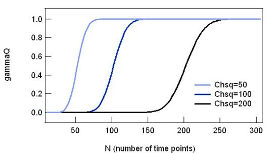
Fig. 2-7-1 gammaQ behaviour

3. Work Flow

3.1. Installing the FRAP Program in the IGORPro

File à Open File à Procedure… à (select the file “K_FRAPcalcV9.ipf”) then click “Compile” at the left-bottom corner of the opened window “K_FRAPcalcV9.ipf”. You will see a new menu ‘Frap Calc’ after compiling the program (fig. 3-1).

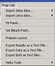
Fig. 3-1 ‘FrapCalc’ menu

3.2. Importing Frap Data

Zeiss and Leica each have their own data output format. The program can import both formats, but the arrangement of data is various. Four different types of fluorescence intensity sampling are possible from FRAP experiments (see 2.1 and 2.2 for more detail) and how they are ordered depends on the user. (Update: Olympus, Excel sheet, and Tab delimited data became available to import , but will not add further explanation since the procedure is similar to Zeiss or Leica)

(a) FRAP ROI time series

(b) Reference or Cell Part ROI time series

(d) Base ROI time series

+ Data file also contains time point data. We call this “Time”.

The program has a list of typical arrangements for each company’s data format[10].

3.2.1 Zeiss Data Format

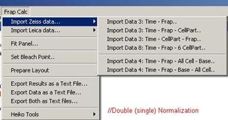
Fig. 3-2 Zeiss data importing

6 different types of data alignments are possible now.

-. 2 columns: Time – Frap

-. 3 columns: Time – FRAP – Cell Part

-. 3 columns: Time – Cell Part – FRAP

-. 8 columns: Time – FRAP – 6 x Cell Part

-. 4 columns: Time – FRAP – All Cell – Base

-. 4 columns: Time – FRAP – Base – All Cell

3.2.2 Leica Data Format

In Leica data format, data for each ROI is separately written in different places within the file. Data first starts with ROI1, with several columns containing frame number, time, channel1 and then channel 2 if there is. Then below ROI1, next ROI2 starts. For this reason, one must select either single or double channel data structure.

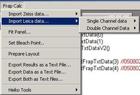
Fig.3-3 Leica Data Importing

In case of single channel data, you have two choice for the data structure.

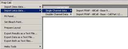
Fig. 3-4

-. single channel with three ROIs: FRAP – AllCell – Base

-. single channel with four ROIs: FRAP – AllCell – Base – Cell Part

In case of double channel data, either channel 1 or channel 2 must be selected to tell the program which channel is actually the frapped channel. If Channel 1 is the frapped channel then do

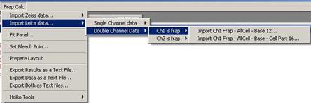
Fig. 3-5

If channel two is the frapped channel then do

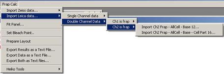
Fig. 3-6

In both cases , two types of ROI sets are available.

- three ROIs: FRAP – AllCell – Base

- four ROIs: FRAP – AllCell – Base – Cell Part

In all cases, when you select one of the importing command, pop up window will appear (Fig. 3-7).

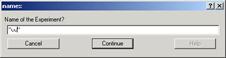
Fig.3-7

Input any name you like for the experiment (but do not start the name with a number & no space within the name!!). Click “Continue”. Another window pops up to select the data file. Select, and then press OK. Almost immediately, a table and a graph like figure 3-5 will appear. This is the original data. If you selected a data format that does not matches with what you have selected in the menu, then importing is aborted and a warning window appears, telling you how many columns the file contains.

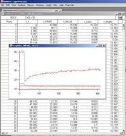
Fig. 3-8

Figure 3-8 shows a snapshot of screen when you import Leica data file with full set of ROI.

3.3. Opening and Using Fit Panel

3.3.1. Open Fit Panel Frap calc à Fit Panel… This will create a panel shown in the figure 3-6.

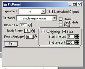
figure 3-6

3.3.2. Most important step before actual fitting is user-input of the FRAP bleach point. Check through the table that was automatically opened when you import the file and find out the point number (not time) of the bleaching. Note that the numbering of cells start from 0, so 6th cell would be cell number 5, and if that is the time point of bleaching, you should set the bleaching time point to 5. Then input the number at the “Bleach Pnt” field[11]. You can toggle the number by clicking the up-down arrow at the right side of the input window.

3.3.3. Using drop-down menu titled ‘experiment’ at the top of the panel, select one of the experiment you imported and named.

3.3.4. Using drop-down menu for ‘Fit Model’ at the second row, select one of the model that you are going to fit. Four different models are possible.

- Single exponential chemical reaction model

- Double exponential chemical reaction model

- Ellenberg’s diffusion formula

- Soumpasis’ diffusion model

3.3.5. From three different normalization methods, choose one by checking one of the check boxes beside the “Fit model” drop-down menu. Three different normalization methods are possible:

- Rainer’s method

-Back Multiplication method

- Phair’s method (Double or Single normalization)

Note: Check buttons will be enabled or disabled automatically depending on the fit model you selected. For example, single exponential model enables all three normalization methods but diffusion models are only possible through Phair’s double normalization.

3.3.6. When you select Diffusion models, you must enter the “Frap Width”, the size of the FRAP bleached area in µm. Otherwise resulting diffusion coefficient will be wrong.

3.3.7. Press ‘Fit!’ button at the left-bottom corner of the panel. This will create a new graph (if there is already a graph window for the corresponding experiment, pressing the button will bring that window forward) and do the fitting. The result is as shown in the figure 3-7 (Rainer’s – Single Exponential), figure 3-8 (Back Multiply – Single Exponential), figure 3-9 (Phair – Single Exponential).

Fig. 3-7 Rainer’s – Single Exponential Blue dots are the decay curve (both Whole Cell and Reference data), Red dots are the FRAP data. Light blue curve is the fitted FRAP curve. Yellow dotted curve shows the estimation curve (see 2.x for details). At the top of the graph, residuals of the fitting are plotted. Inadequate model will result a systematic deviations, as you can see in this figure.

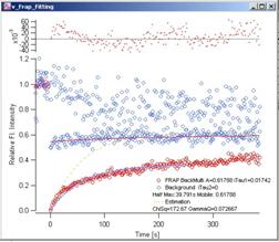
Fig. 3-8 Back Multiply – Single Exponential Blue dots are the decay curve (both Whole Cell and Reference data), Red dots are the FRAP data. Red curve shows the fitting of whole cell data. Light blue curve is the fitted FRAP curve. Yellow dotted curve shows the estimation curve (see 2.x for details). At the top of the graph, fit-residuals

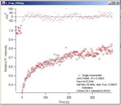
Fig. 3-9 Phair – Single Exponential Red dots are the FRAP data. Light blue curve is the fitted FRAP curve. Decay data are not shown. Yellow dotted curve shows the estimation curve (see 2.x for details). At the top of the graph, fitting residuals are plotted.

3.3.8 Fitted parameters will be indicated in three different places. (1) Within the graph as legends (2) In the history window (3) In the fit Panel. The results printed in the history window looks like figure 3-10.

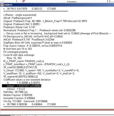
figure 3-10

GammaQ must be first checked to evaluate the fitting (see 2.7). If gammaQ value is less than 0.01, than you must redo fitting either by

(1) Limit the data range for fitting by checking ‘Limit’ check box within the Fit Panel (see fig3-6) and input time points for a desired range. After setting start and end time points, press ‘Fit!’ button again. Alternatively, you can also weight a certain range if you check ‘Weighting’. This will consider the specified range to be 10 times more important than the other parts, in terms of Chi-squared value.

(2) Use other fit models and compare gammaQ value. Larger value is better.

If you have a sufficiently large gammaQ, then results can be used as your data. The last line in the history window is tab delimited in the order of

experiment name – half max – Mobile fraction – immobile fraction – Chi-Square.

You can copy and paste the line to spreadsheet software such as Excel, and each parameter will be pasted separately to single cells.

3.4. Output

3.4.1. To print out graph and fitted parameters, do Frap calc à Prepare Layout. This will create a window called “layout” containing both the graph and the results for printing out.

3.4.2. To export fitted parameters as formatted text file, do Frap calc à Export Results as a text file.

3.4.3. To export frap data as formatted text file, do Frap calc à Export Data as a text file.

3.4.4. To do both 3.4.2. and 3.4.3, do Frap calc à Export Results and Data as a text file.

3.5 Batch Analysis (added: Feb. 2010)

When you have many FRAP experiments done with same condition, you could average those curves and get a better idea of more general recovery curve. In addition this has an advantage: standard deviation at each time point could be calculated and these deviation values could be used as parameter for curve fitting. Less standard deviation would mean that those points are more reliable then the points with larger standard deviation. During fitting, such difference in reliability of the measured value could be reflected to the process of curve optimization (see chi-squared equation, 2-30) Points with less standard deviation are typically at the initial phase of recovery, and these points will be considered more important during the fitting.

IMPORTANT: for averaging curves, you need to do experiments with same timing. Otherwise, batch Fitting (see below) works and you get a list of parameters, but the program stops when it detects that acquired time points are various in the data set. You could use calculated parameters for each curves, maybe average them for summarizing your results.

To do batch analysis, each FRAP data must be saved in separate files in a same folder (currently files should be tab-delimited text file, and the data order should be single channel Zeiss Time-FRAP-AllCell-Base: for additional formats, please ask Kota). Then do the following:

1. FRAP calc -> batchprocessing --beta-- -> Batch import... In the window that pops up, choose a folder where text files with FRAP data are stored and click OK. Then data will be loaded automatically. For each curves, a table with data and a corresponding plot appears. During the import, a list of imported experiment names (names generated from the file names) is created. This list is hidden, but you could see the list by typing the following line in the command window.

print Gfilelist

2. Then FRAP calc -> Fit Panel... In the panel, set the bleaching time point. This bleaching time point will be commonly used for all curves. You could already fit individual curves, but if you are in a hurry, you could proceed to step 3.

3. Finally, FRAP calc -> batch processing --beta-- -> Batch Fit. You will see that each individual data is curve-fitted first. Then a plot with averaged curve appears at last. Error bars are added to the curve, so it should be visually distinguishable from other plots. Fit results (parameters) are shown in the plot, history and at the bottom of panel.

4. In the panel, you could change the fit model and/or normalization methods, just like singe curve fitting in the panel. Then you could do the "batch fit" again to test the goodness of fit of different models.

Figure 3-11. Batch analysis, averaged curve fitting.

4. Appendix

A. Data Format Codes

+ 1111 () 0 FRAP + Whole Cell + Reference + Base

+ 1101 () 1 FRAP + Whole Cell + Base

- 1011 () 2 FRAP + Reference + Base

- 1100 () 3 FRAP + Whole Cell

+ 1010 () 4 FRAP + Reference

- 1001 () 5 FRAP + Base

+ 1000 () 6 FRAP

B. Fit Method Codes

0: Rainer - single exponential

1: BackGroundMultiply-single exponential

2: BackGroundMultiply-double exponential

4: (back multiply Ellenberg diffusion)

5: (back multiply Soumpasis)

6: Double Normalization, single exponential

7: Double Normalization, double exponential

8: Double Normalization Ellenberg

9: Double Normalization Soumpasis

C. Point Number and its content in FittingParameterWave

0: fit method

1: normalized

2: width

3: background exists

4: flatback

5: BackGround_Timpoint0

6: GapRatio

7: I_prebleachBack

8: I_prebleachFrap

9: I_bleachfrap

10: backamplitude

11: backtau

12: backy0

15: WholeCell_Exists

16: Ref_Exists

17: Base_Exists

5. References

Ellenberg, J., Siggia, E. D., Moreira, J. E., Smith, C. L., Presley, J. F., Worman, H. J. and Lippincott-Schwartz, J. (1997). Nuclear membrane dynamics and reassembly in living cells: targeting of an inner nuclear membrane protein in interphase and mitosis. J Cell Biol 138, 1193-206.

Jacquez, J. A. (1972). Compartmental analysis in biology and medicine: Elsevier.

Phair, R. D., Gorski, S. A. and Misteli, T. (2004). Measurement of dynamic protein binding to chromatin in vivo, using photobleaching microscopy. Methods Enzymol 375, 393-414.

Soumpasis, D. M. (1983). Theoretical analysis of fluorescence photobleaching recovery experiments. Biophys J 41, 95-7.

Sprague, B. L. and McNally, J. G. (2005). FRAP analysis of binding: proper and fitting. Trends Cell Biol 15, 84-91.

Sprague, B. L., Pego, R. L., Stavreva, D. A. and McNally, J. G. (2004). Analysis of binding reactions by fluorescence recovery after photobleaching. Biophys J 86, 3473-95.

Acknowledgements

I thank Martin Offerdinger (Div. Cell Biology, Biocenter Medical Uni. Innsbruck) for finding out mistakes in formula (2-3) for the normalization of diffusion recovery (but I should tell you, the original code was correct, it was only the formula in this document!). I also thank Jim Prouty (Wavemetrics) for correcting the code for IgorPro ver6.0.

[1] When base-ROI measurement is not available, the program omits the subtraction of off-set value.

[2] This section matters only for the “Rainer’s fitting”

[3] If you are FRAP-bleaching large portion of the total fluorescence, this becomes evident with the acquisition decay curve. There will be a sharp decrease in the fluorescence after you FRAP-bleach. This decrease is not due to the acquisition bleaching but for the reason (b) I mentioned above.

[4] Function name: K_estGapRFromOrigAllcell(flatback)

[5] Function Name: K_estGapRFromOrigRef(flatback)

[6] For the calculation of gap ratio, non-normalized, original decay reference curve is used. This is because with normalized curve, the value could be negative. Since we do not know the intensity offset (baseline), we use 0 in the original curve as the offset value.

[7] Note that these formulas are a bit different from the original in Axelrod et al (1974) or Soumpasis (1982). τD (in their paper) = τ/4 (in Sprague and this document).

[8] in IgorPro, this is gammq function and uses Numerical Recipe in C third ed. algorithm.

[9] In the program, one can control the range of FRAP curve to fit using ‘Fit Panel’. See ‘Work Flow’.

[10] For extending the program to enable importing different data arrangements, ask Kota. It’s not so difficult.

[11] The bleaching time point can also be set from the menu Frap calc à Set Bleach Point