Developmental Biology, Behavior Module
Nov. 25, 2009 Kota Miura (Centre for Molecular and Cellular Imaging. EMBL)
Aim: Analyze Platynereis larvae phototaxis behavior
Methods:
Larvae distribute randomly in dark, but when light is laterally irradiated larvae accumulate on brighter side due to phototactic swimming of larvae. We evaluate this behavior in two ways.
1. Evaluation of Phototaxis by population (counting)
2. Evaluation of Phototaxis individually (tracking)
Protocol
1. Software Installation
1-1 Download and Install ImageJ
For the course, use the following link, and download the file directly on your desktop.
Original: go to http://rsb.info.nih.gov/ij/docs/install/windows.html
Download ImageJ zipped package (one that is packaged with JRE)
If OS is Linux: http://rsb.info.nih.gov/ij/docs/install/linux.html
1-2. If excel is not installed, download and install OpenOffice Calc
2. Evaluation of Phototactic Behavior by Population
Degree of this phototactic behavior can be evaluated plotting distribution of larvae along axis of light irradiation. For this, we use "particle analysis" function in ImageJ.
Assignment: Compare the degree of phototaxis by comparing position of larvae (1) in Dark, (2) at least three time points after light irradiation. Plot two-bar graph for dark and each time points after the light irradiation. Discuss the effect of drug treatments. If you have time, estimate the “Phototaxis Velocity”.
Work Flow:
2.1. Open image stack with larvae swimming. Since these stacks are “Inverted LUT” we want a normal LUT. For this, do
[Image -> Look Up Tables -> Invert LUT]
then image intensity inverts. Then do
[Edit -> Invert]
ImageJ asks you if you want to process all frames. Click OK. The stack then looks like the original, but now the stack is with normal look-up table.
2.2. Separate stack to dark and light irradiation phases.
If stack contains both dark and light irradiation phase, separate the stack in two dark stack and light stack (this is required for background subtraction, since background should be approximately same intensity). For this, you could "duplicate" dark phase frame and light irradiated phase. First, go through stack using “,” (rewind) “.” (forward) and find out at which frame light irradiation starts. For example, if you find that light irradiation starts from frame 130 in a stack with 750 frames, do
[Image -> Duplicate…]
Then there will be a dialogue panel that looks like below.
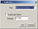
Change the “range” to 1-130 and check “duplicate stack”
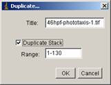
and then click OK button. This will generate another window, with frames only during dark. If you duplicate 131-750, this second duplicate will contain only light phase.
Activate a stack window by clicking its title bar. Then do
[Image -> Stacks -> Z Project…]
Then a dialogue panel appears. Choose “Average Intensity” from projection Type drop-down menu, and click OK.
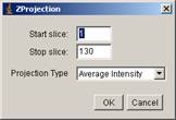
This will create another window with single frame. We call this background image (background).
Then we subtract background from the original stack (stack - background image).
[Process -> Image Calculator…]
then a dialogue panel appears.
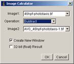
As Image1, choose the stack. Then Operation should be “Subtraction” and Iamge2 should be the background image. Check “Create New Window”. click OK. Click yes for “Process all…?”. A new stack with title “Result …” is the back-subtracted stack.
2.4. Particle analysis.
2.4.1. Blur the image a bit to remove noise.
[Process -> Filters -> Gaussian Blur].
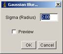
Sigma should be 2.0. Then OK. Process all frames.
2.4.2. Set Measurements.
Measured parameters should be set.
[Analyze -> set measurements].
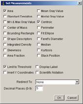
Check “Area”, “Centroid” and “Limit to threshold”. Click OK.
2.4.3 Particle Analysis.
First, particles must be thresholded.
[Image -> Adjust -> Threshold..]
Adjust the lower threshold so that larvae are nicely selected.
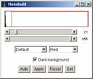
** note: If you see many larvae overlapping, click “Apply” in threshold panel. This will generate a black and white image. then do [Image -> binary -> Watershed] to separate overlapping particles. Do the threshold again.
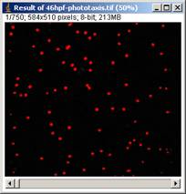
While you see the selected larvae in red, do
[Analysis -> Analyze Particles…]
In the dialogue panel, set parameters as below.
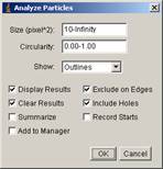
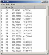
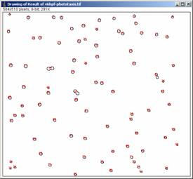
Click OK, and when the program asks you whether to process all frames, click NO. You will see two windows newly appeared, “results” and “Drawing of …”
2.5 Plotting data
Plot distributions directly from results window. In the “Results” window, do
[Edit -> Distribution…]
and in the panel, select “X” as parameter, and specify bins to 10, range 0-600 (max of range should be the width of the image, so it could be different, not 600).
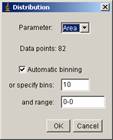
and click OK.
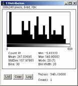
Dark
Distribution can be exported as a list (Click “List” in the distribution panel such as above, and copy & paste the table into other software. The table could also be saved as a tab-delimited text file and imported into Excel or OpenOffice calc).
--- plotting in spread sheet ---
Use spread sheet software and evaluate the results, and discuss the phototaxis with different drug treatments.
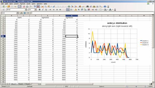
Distribution such as above can be simplified to two-bar plots (left side vs right side population). This could be done, when you do “distribution” in ImageJ, assign bin = 2.
2.6 Estimation of Phototaxis Velocity
3. Evaluation of Phototaxis by Individual Tracking.
By tracking individual larvae, we get XY coordinates of the larvae in time-lapse movies. These series of XY coordinates can be used to calculate the parameters of movement to characterize the movement. Since larvae swim by propulsion (forward movement) and rotation (rotation about its long axis), we can simplify the movement as an association of two movement vectors: forward vector and tangential vector.
3.1 Manual Tracking
Manual tracking is always convenient. Even with very bad-quality images, it will be possible to get track data. Bad side is that it takes time and work loads.
3.1.1. Open stack. [File -> Open]
3.1.2. [Plugins -> Course -> Manual Tracking]: a panel pops up.
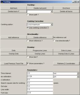
3.1.3 Start manual tracking by clicking “Add track” and end tracking by “End track” (frames proceeds automatically as you click). After finishing the track, you could click “Add track” again to track another one. Coordinates will be recorded in the results window.
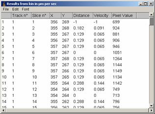
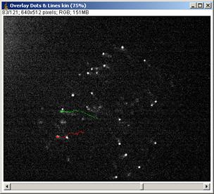
3.1.4 After tracking several larvae, show tracks by clicking “Overlay Dots & Lines”. If you think its OK, then eave the results by [File -> Save as] (menu in the Results window ) or you could directly copy and paste to spread sheet software.
3.1.5 Do analysis as assigned in 3.3 (see below).
3.2. Automated Tracking
We use Particle Tracker Plugin for automated tracking of larvae.
Automatic tracking reduces the workloads of the researcher, enabling them to deal with a huge amount of data. Statistical treatments can then be more reliable. In addition, the results can be regarded more objective than manual tracking. Automatic tracking is an optional function that can be added onto some imaging software. However, these readily available functions are not adaptable for all analyses since the characteristics of target objects in biological research vary greatly. Especially when the target object changes shape over time, further difficulty arises. For these reasons, automatic tracking often requires custom programs. In ImageJ, Pascal-like macro programming is possible and there are many programming functions that enable such automated segmentation and position measurements.
Work Flow
3.2.0 Open stack. [File -> Open]
3.2.1 LUT conversion and background subtraction
Do as instructed in 2.1 and 2.3.
3.2.2 Tracking: [Plugins -> Course -> Particle Detector & tracker: Particle Tracker]. First, adjust parameters (radius, cutoff, percentile) to find out a combination of parameters that detects larvae well enough in my case, radius = 5, cutoff = 0, percentile = 0.2 yielded best detection. Then set parameters for linking: in my case, Link range = 3, displacement = 20 yielded best results, but this linking could be redone easily after tracking so take this easy.
3.2.3 Save tab-delimited text file (tracks)
3.2.4 re-importing results to ImageJ
Inspect tracks, choose successful ones
3.2.5 Do analysis as assigned in 3.3 (see below).
Assignments: Track swimming larvae. Do the following analysis and discuss the results.
(a) plot instantaneous velocity vs time of several of sampled larvae
(b) calculate mean velocity of each larvae
(c) calculate mean velocity of all sampled larvae
(d) plot instantaneous phototaxis velocity vs time
(e) calculate mean phototaxis velocity of each larvae
(f) calculate mean phototaxis velocity of all sampled larvae
(g) plot instantaneous direction (cosθt) vs time
(h) calculate mean direction of each larvae
(i) calculate mean direction of all sampled larvae
(j) calculate swimming efficiency of each larvae
(k) calculate average swimming efficiency of all sampled larvae
Parameters: Track can be represented as (x0, y0), (x1, y1) …. (xt, yt) …(xn, yn). Then we can calculate movement parameters as follows.
Instantaneous vector: at time point t.
![]()
Instantaneous Velocity: displacement of larvae between frame t and t+1.
![]()
Since these values has scales of pixels and frames, unit of this velocity is [pixels/frame]. To convert this to SI unit, and if spatial resolution is f1 [μm / pixel] and f2 [sec / frame],
Vt in SI [μm / sec] = f1 / f2 (Vt [pixels/frame])
Mean Velocity: average of all instantaneous velocity from a track (same for the unit conversion).
 (total displacement divided
by number of displacement)
(total displacement divided
by number of displacement)
Instantaneous Phototaxis Vector and Velocity: Velocity along light axis
if light is irradiated from left side, then phototaxis vector (movement that contributes to phototaxis) is simply omitting the y-component of movement.
![]()
then instantaneous phototaxis velocity is
![]()
* if light is irradiated from right side, then -1 is not multiplied.
Mean Phototaxis velocity:
![]()
Tangential Vector: We assume that the forward vector is similar to previous time point vector and define the tangential vector as follows:
![]()
![]() : Instantaneous
vector at time point t.
: Instantaneous
vector at time point t.
![]() : Instantaneous vector at time
point t-1.
: Instantaneous vector at time
point t-1.
Magnitude of tangential vector corresponds to the degree of force generated by larvae for turning.
![]()
Instantaneous Direction θt: angle made between ![]() and
and ![]()
since we know that for ![]() and
and ![]() internal
product is
internal
product is
![]()
and also
![]()
instantaneous direction θt could be calculated by

(-1 < cos θt < 1)
Swimming Efficiency: Net Displacement divided by total displacement
Appendix I: Phototaxis Velocity
In square chamber (1cm x 1cm) used for recording the swimming behavior of larvae, there are approximately 40 larvae within the image field. We assume that this number is approximately constant.
When there is no environmental bias, numbers of larvae in the left half (LH) and right half (RH) of the chamber are mostly similar because the swimming is randomly directed. When light is irradiated from the right side of the chamber, swimming direction becomes biased towards the right side that the number of larvae in RH becomes larger than that in the LH. The speed of the increase of the larvae number in the RH depends on the "net flux" of larvae from LH to RH.
![]()
where Na is the total number of larvae. This is because the mean value of Vx (Velocity component along x axis) is 0.
When light is irradiated, mean value of Vx become positive because the swimming direction of larvae are now directed towards Right side. We call this biased value as
![]()
The time it takes for all the larvae in the LH to change there place in RH (we call this time as tduration)*1 is then
![]()
where w is the width of the chamber (in average, larvae in LH travels distance of w/2 in x-direction for changing their location to RH). Then
![]() (1)
(1)
where Jp is the Phototaxis Flux (number of larvae / time) that causes net flux from RH to LH. Since the increase of the larvae in RH is directly proportional to Jp, change in Nlh follows the following simple formula:
![]()
By fitting the slope of the increasing Nrh(t) in experiment, the slope Jp could be estimated. Vp could then be derived using the formula (1).
* Since larvae are also moving randomly, there is no perfect relocation of all larvae but we assume that this dynamic balance is included in Vp.