Manual: Vector Field Analysis
Kota Miura (miura at embl dot de)
Centre for
Molecular and Cellular Imaging, EMBL Heidelberg
Tel. +49 6221
387 404
Document Date: 2010-03-10
Main Features
- IgorPro (Wavemetrics)[1]
Procedure.
- Optical Estimation by temporal local optimization.
- Plotting of vectors in the original video frame.
- Filtering of the vectors by image intensity,
velocity and direction.
- Image masking.
- Histograms of velocity, directionality.
- Calculation of protein flow rates.
TOC
1. Introduction
2. Work Flow
3. Appendix 1: Checking the average intensity fluctuation
Appendix 2: Enhancing
Contrast
Appendix 3: Checking
the shutter timings
Appendix 4: Walking average
Appendix 5: Preparing Image Mask
------------------------------------------------------------------------------------------------------
1. Introduction
The
vector field analysis program uses an algorithm that is called the optical flow
estimation (Teklap,
1995). Optical flow is “the distribution
of apparent velocities of movement of brightness patterns in an image” (Horn and Schunck,
1981). In video sequences the projection
of temporal axis to the x-y plane
results in an optical flow image. Since the optical flow is a result of the
movement, it contains information on movement speed and direction. The optical
flow estimation recovers these quantitative measures of the movement, which
enables the statistical treatments of all movement that occurs in the sequence.
A velocity vector field is the calculation result in which every movement,
namely speed and direction, within the sequence is mapped. The largest
difference to the other tracking technique is that this operation does not
require the segmentation step.
Optical flow detection can be categorized into two
types in terms of basic algorithm: the matching
method and the gradient method.
In the matching method, displacement
is measured by searching for a particular region in the consecutive frame by
matching the pattern of the previous frame. In the gradient method, optical flow is detected by assuming no changes in
the signal intensity pattern at different time points and by using equations
that correlate the spatial and temporal intensity gradient. This program uses
the gradient method. Details are described elsewhere (Miura, 2005).
Briefly,
a general assumption in the gradient method is that the
total intensity of the image sequence is constant:
![]() (1)
(1)
v(u,v)= v(![]() ,
,![]() ) (2)
) (2)
Where I(x,y,t) is
the intensity distribution of the image and v is the optical flow vector. The equation (1) links the partial derivatives of the brightness pattern of the
image sequence and the optical flow velocity. Since there are two unknowns,
another constraint is required.
The temporal local optimization
method (TLO) used in this program assumes that the optical flow field is
constant temporally (Fig. 6) (Nomura et al., 1991).
![]() (3)
(3)
The constant vector can be assumed
for N frames. Then for a stack with
frames ![]() , following error function can be generated:
, following error function can be generated:
![]() (4)
(4)
By the least
squared method, v(u,v)
can be determined by two equations![]() and
and ![]() .
.
A series of tiff-format image frames
is converted to a stack, which is then treated as a three-dimensional matrix I(x,y,t).
Partial derivatives of the image sequence must be first calculated as seen in
equations 1 and 4. There are three popular ways for obtaining the first-order
partial derivatives[2];
Sobel kernel, Roberts kernel and Prewitt kernel (also is called two-point
central difference kernel). The Prewitt kernel was used as follows:
 (5a)
(5a)
 (5b)
(5b)
![]() (5c)
(5c)
2.1. Preprocessing of image stack before doing the
vector field analysis
For a
successful analysis, following preprocessings are
recommended:
- Check average intensity
fluctuation of the sequence (recommended: see Appendix 1).
- Generate “Image Mask” using ImageJ
(Fig. 1: see Appendix 5). You might not need this if
there is no background area in the image.

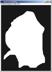
Fig.1 The “image filter” should look something like
this. White area will be calculated for vector field. Such masking is required
since noise in the background causes tiny vectors that contaminate the
measurements.
- Determine the range of frames
to use for the Vector Field analysis by inspecting different time points
of the stack. Check the shutter timing as well (App.3).
A large fluctuation in the image intensity, avoid using those time points.
- It is strongly recommended to do
the walking-averaging of the sequence to decrease the noise (App. 4).
- If required, adjust contrast (App.2).
2.2. Setting up the Vector Filed Program in the IGORPro (Compiling)
Do [File à
Open File à Procedure…] and select the file “vec9.ipf”
somewhere you know. Then click “Compile”
at the left-bottom corner of the opened procedure window. In the menu bar,
“Vector field” and “Directionality” appears.
* Tip: If compile does not work, it could be that other procedure files
(.ipf files) are not in the reference path. Check
“User Procedures” folder, and see if the folder containing Vec9.ipf is linked
or copied in that folder.
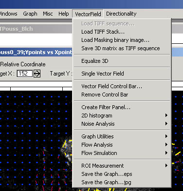
Vector Field analysis menu
C. Vector Field Analysis
1. Import a image stack by [VectorField à Load Tiff Stack].
2. Import the image mask in the Vector Filed Analysis Program in the IGORPro. [VectorField à Load Masking binary image...]
*Image Filter can be inverted by VectorField à 2D histogram à Invert Mask.
This function is sometimes convenient since one might prepare a mask which
selects only the background of the sequence.
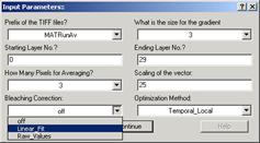
3. Calculate the vector field by [VectorField à Single Vector Field]. In a window that pops-up, select the tiff-stack,
input the frame range (normally, I use 30 frames by experience that this is
sufficient number of frames). Choose Bleaching Correction “linear fit”, if there is a bleaching of the sequence. Other
parameters do not have to be changed now. “Averaging” and “Scaling” could be
adjusted later after the main calculation.
It takes a while to calculate the vector field. While then there will be
a rotating-disc icon indicating that the calculation is going on, at the right
bottom corner of the IgorPro window.

Rotating Disc icon
If this calculation is first time in the current igor-experiment,
then IgorPro asks you for a path’

Click ‘Browse’ button and select “NoiseParameter”
folder within Vec9 folder.
After the calculation, a new Vector Field window appears.

There will be also two new windows, one for the speed histogram and
another for the direction histogram.
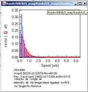
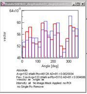
Speed histogram Direction histogram
4. To decrease the visualized vectors, adjust the vector scaling and
averaging higher. To do so, activate the vector field window and then do [VectorField à
Vector Field Control Bar...]. This will append a header bar at the top of the vector field plot, and
averaging and scaling of vectors could be adjusted interactively.
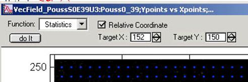
5. OPTIONAL: Within the Vector Field Control Bar, select “Statistics”
from the pull-down menu. Check “relative”, then input the coordinates for the
reference points. The coordinates can be measured easily by making a target ROI
in the vector field, right click the mouse button within that ROI. A menu will
appear and choose “V_show_ROI_center”.
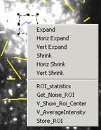
The centroid coordinates of the selected ROI will be printed in the
History window. Input those values in “TargetX” and “TargetY”. Clicking “Do it” button will change the
measurement of direction of the vectors against the reference point.
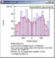
The direction histogram changes its range from 0 - 360º to -180º -
+180º. In the latter case, 0º is directed towards the reference point, and
±180º is directed away from the reference point.
6. OPTIONAL: Filtering. If vector field is influenced by noise largely,
these noise derived information must be removed from the measurement. To do so,
do [VectorField
à
Create Filter Panel...].
This then pops up a window titled “Filter Panel”. There are several types of
filters and you can set their parameter to remove noise derived vectors.

a. Find the optimum lower and higher limit for the intensity filter
(compare the original movie and the vector field). Input the values within the
Filter Panel. For selecting intensity range, threshold function in ImageJ is
useful [Image-> adjust ->
threshold].
b. Find the “speed of noise” from the back ground and set the lower
limit for the speed detection. Input the value in the Filter Panel.
c. Set the image-filter by checking the “Mask” check box. A dialogue
window will appear. Select the Image Mask from the pull down menu.
d. Don’t forget to check the “Display Filtered” check box.
e. Click “Do it” to execute the filtering. After the filtering is done,
yellow vectors will appear, which are the vectors after the filtering.
Statistics will also change, showing only the results from those yellow
vectors.
f. Filtering parameters can be changed and re-calculated.
7. Flow Rate calculation.
a. Check the background intensity. Move the curser to the background
region of the vector field, click right mouse button and select “V_AverageIntensity” form the menu. The average background
intensity will appear in the command window.
b. Set background intensity by VectorField à Flow Analysis à Set Background
Intensity.
c. Do the analysis by VectorField à Flow Analysis à Calculate Flow.
New graphs will appear.
Appendix 1: Checking
the average intensity fluctuation.
Dealing with Image Sequences with Blinking
(Fluctuation of the fl. Intensity)
One could
measure the temporal changes in the average intensity of frames in the
following way.
First, open the
stack that you want to measure.
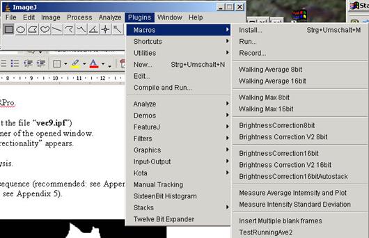
Then a macro
program should be installed.
[Plugins à
Macros à Install…]
Then a popup
window appears and a file called “StackManager.txt”
must be chosen from wherever it is saved. This file could be downloaded from
http://cmci.embl.de/dls/StackManager.ijm
as well (right
click and “save link as”).
You will see
new commands in the Macros menu [Plugins -> Macros -> …].
Activate the
Stack window by clicking the title bar, and then select “Measure Average Intensity and Plot” form the macro menu. The
program goes through the sequence once and then there will be a new window that
looks like below.

This plot shows
how the average intensity of your sequence changes from frame to frame. The
average intensity is decreasing, because there is a slight acquisition-photobleaching
of the fluorescence.
In some cases,
the intensity fluctuates largely. This could be caused by several reasons such
as unstable light source (this happens a lot with old lamps) or changes in the
focus plane. In any case, avoid using such a sequence, or use only a part of
the sequence with a constant intensity (or with a constant photo-bleaching rate)
Appendix 2: Enhancing contrast and down scaling from 16 bit to 8bit
This
explanation applies to 16-bit image sequences.
Open 16bit Tiff
Sequence as a Stack in ImageJ.
Select a frame
at a position about 2/3rd of the whole sequence.
Check that the
frame is not extraordinarily bright or dark.
[Analyze à
Histogram]
In a window
that pops up, you see an intensity histogram of the image. In general, there is
a narrow peak.
Since this is a
16bit image, Grayscale has 65536 (=216) steps between black(0) and
white(65535) You need to down scale this and set a full rage in 8 bit, which
consists of 256 (=28) steps.
For example, if
histogram of a frame distributes in a range of pixel values between 82 and 1009,
it means that there are about 900 gray value steps in the image. Although with
such a wide dynamic range, the largest peak tends to be in a much narrower
range. To determine the intensity range where concerned signal is distributed,
you should the peak must be examined carefully to know if that peak is really
your object, or simply background. For this, you could use two different histogram
tools: interactive pixel value reading and numerical out put.
Interactive pixel value reading: Try moving your curser position above the histogram
window using your mouse. If you let your curser move across the histogram, you
will notice that “Value” at the bottom of the histogram changes. “Value” means
the Gray value, the whiteness of the pixels. “Count” shows the number of pixels
with that gray value. e.g. if your curser is at “Value” 328 and “Count” is 26, it
means that the number of pixels with a gray value of 328 in the image is 26
pixels. As you move your curser closer to the peak, “Count” starts to increase.
e.g. the “Value” is 165, “Count” is 435, and so on. Compare the value readout
and actual pixels values in the image to figure out the background intensity.
As further
example, if the tail of the peak is approximately at the position “Value”=144
(Fig. A2-1). The tail in the other side can be also determined in a same way.
Let’s say “Value”=86 as the other end.
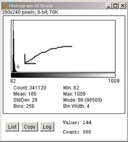
Fig. A2-1
Numerical readout: Click the “List” button in the histogram window. A
list of number appears. This is the actual values of the histogram. The first
column is the “Value” and the second column is the corresponding “Count” By
examining the histogram values, the approximate steps that contain the peak
position can be determined.
16bit images
could only be contrast enhanced during conversion to 8-bit.
[Image à
Adjust à Brightness/Contrast]
This will open a
small window with a pixel intensity histogram. Click “set” button. A small
window pops up. Set the “Minimum Displayed Value” to 86 and the “maximum
displayed value” to 144. Now you see that the Image is contrast enhanced. But
don’t be satisfied. The process down to here have only changed how the image
is displayed (LUT), not the image itself. There has been no treatment to
the data. This is an important point, since in many case, one only changes how
they are displayed (or how they appear on the monitor screen) however this is
not a real processing.
To process the
image, you need to
[Image à
Type à
8bit]
This operation converts
the image data. You can check that by opening the histogram again.
[Analyze à
Histogram]
.. and you see
that the peak is nicely distributed between the value 0 and 255.

Fig. A2-2
Appendix 3: Checking the shutter timings.
Some sequences
contain “blinking” of the frames. This could be due to
1) Light-source
shutter is unstable.
2) Camera
shutter is unstable.
3) Light source
itself is blinking.
4) focusing
position changed.
For the camera
shutter stableness, one can go back to the shutter log (“time stamps”) and
check if the sequence was taken with a constant shutter timings. Here is an
example.

dt plot generated from the “.tim” file.
For the possibility of that the 3) light source itself was blinking,
this seems to be not convincing because increase/decrease of the bright ness is
rather slow. The blinking of the light source has a higher frequency.
Walking averaging of a image sequence converts each frame of the
sequence to an average of successive frames. à ImageJ macro (StackManager.txt) ask Kota for a copy.
After installing the macro, ImageJ macro menu looks like this:
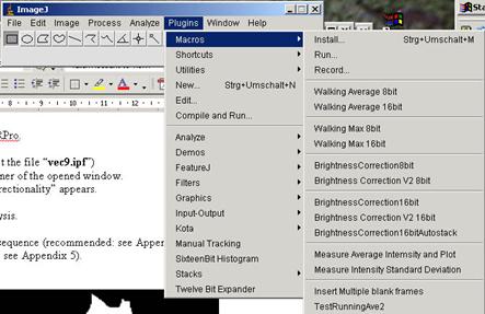
If the stack is 8bit, choose “Walking average 8 bit” If 16bit, choose
“Walking average 16 bit”. Then a pop-up window appears:
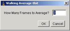
Input number of frames that you want to average, then click “OK”. A new
stack appears that is walking averaged.
Appendix
5: Generating a Image Mask for Vector field.
To make image mask, you need to use ImageJ. First, you must make two
copies of a frame in the sequence you want to analyze. This can be done by
[Image -> Duplicate…]
This will create a copy of the frame in the stack. If image is not 8-bit,
then convert the image to 8 bit by
[Image -> Type -> 8bit]
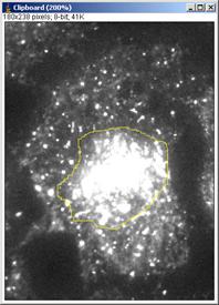
Using this duplicated frame, you need to trace the edge of the cell. This
is done by selecting freehand tool. Click the freehand ROI icon in the ImageJ
menu bar.

Then trace the cell edge like figure shown below left side image.
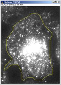
Then after tracing, do
[Edit à Fill]
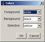
Tip: If inside area of the ROI do not become white, then check color
option by [Edit -> Options -> Color…]. Check that the color assignment
shown in the window appeared is like the one shown below.
Then
[Edit à Clear outside]
This will fill black in the outside area of selected ROI. By these last
two steps, image should have become black and white.
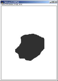
OPTIONAL: masking area inside cell.
Sometimes signal is too high inside cell and this interferes with your
vector analysis. In such a case, another mask could be prepared to mask that
high-intensity area, and combine it with the cell edge mask prepared above. You
first make another duplicate of a frame by [image
-> duplicate]. Then Trace the high intensity area, and convert them to
black ad white just like the first one.

Since we do not want to measure the white area, we invert the image so
that the selected area becomes black.
[Edit
à
Invert]
finally, use Image calculator to combine two masks.
[Process
à
Image Calculator…]
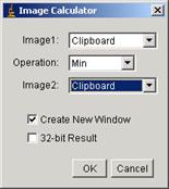
Select the first clipboard as image 1 and the second clipboard as the
image 2. Operation is “Min”. Then the image mask is created and can be imported
from IgorPro.

References
Horn, B. K. P. and Schunck,
B. G. (1981). Determining Optical Flow. Artificial
Intelligence 17, 185-203.
Miura,
K. (2005). Tracking Movement in Cell Biology. In Advances in Biochemical Engineering/Biotechnology, vol. 95 (ed. J. Rietdorf), pp. 267. Heidelberg:
Springer Verlag.
Nomura,
A., Miike, H. and Koga, K. (1991). Field theory approach for determining optical flow. Pattern Recog. Lett. 12,
183-190.
Teklap, M.
(1995). Digital Video Processing. Englewood Cliffs, N.J.: Prentice Hall.